Parametrization of a New Polymer
Version: 1.0.0
Contributed by: @ricalessandri.
Files required and worked examples for this tutorial can be downloaded here.
Table of contents
1) Generate atomistic reference data
3) Generate the CG mapped trajectory from the atomistic simulation
4) Create the initial CG itp and tpr files
5) Generate target CG distributions from the CG mapped trajectory
7) Optimize CG bonded parameters
Introduction
In this tutorial, we will discuss how to build a Martini 3 topology for a new polymer. The aim is to have a pragmatic description of the Martini 3 coarse-graining (CGing) principles described in Refs. [1] and [2], which follow the main ideas outlined in the seminal Martini 2 work [3]. Finally, this tutorial will pay attention to aspects that are specific to polymer model parametrization.
This tutorial is based on the analogous Martini 3 tutorial for parametrizing a new small molecule. We will use as an example polyethylene oxide (PEO), and make use of Gromacs versions 2019.x or later.

1) Generate atomistic reference data
We will need atomistic reference data to extract bonded parameters for the CG model. Note that we will need all the hydrogen atoms to extract bond lengths further down this tutorial, so make sure that your atomistic structure contains all the hydrogens.
Here, we will use the LigParGen server [4] as a way to obtain an atomistic (or all-atom, AA) structure and molecule topology based on the OPLS-AA force field, but of course feel free to use your favorite atomistic force field. Other web-based services such as the automated topology builder (ATB) or CHARMM-GUI can also be used to obtain reference topologies based on other AA force fields. Another important option is to look in the literature for atomistic studies of the molecule you want to parametrize: if you are lucky, somebody might have already published a validated atomistic force field for the molecule, which you can then use to create reference atomistic simulations.
Start by feeding the SMILES string for a tetramer of PEO (namely, COCCOCCOCCOC) to the LigParGen server,
and pick the “1.14*CM1A-LBCC (Neutral molecules)” charge model (nothing special about this choice of charge model).
We choose a tetramer of the polymer, a short polymer containing 4 repeat units,
because this is the smallest amount of repeat units that allows us to define
bonds (between pair of CG sites), angles (between triplets of CG sites), and dihedrals (between the 4 CG sites).
After submitting the molecule on LigParGen, the server will generate input parameters for several molecular dynamics (MD) packages.
Download the structure file (PDB) as well as the OPLS-AA topology in the GROMACS format (TOP) and rename
them PEO4_LigParGen.pdb and PEO4_LigParGen.itp, respectively. You can now unzip the zip archive provided:
unzip files-m3-newpoly.zip
which contains a folder called PEO4-in-vacuum that contains some template folders and useful scripts.
We will assume that you will be carrying out the tutorial using this folder structure and scripts. Note that the archive
contains also a folder called PEO4-worked where you will find a worked version of the tutorial.
This might be useful to use as reference to compare your files (e.g., to compare the PEO4_LigParGen.itp
you obtained with the one you find in PEO4-worked/1_AA-reference).
We can now move to the first subfolder, 1_AA-reference, and copy over the files you just obtained from the LigParGen server:
cd     PEO4-in-vacuum/1_AA-reference
[move here the obtained PEO4_LigParGen.pdb and PEO4_LigParGen.itp files]
Input files obtained from LigParGen come with unknown (UNK) residue names. Before launching the AA MD simulation,
we will substitute the UNK residue name by PEO4. To do so, open the PEO4_LigParGen.pdb with your text editor of choice
and replace the UNK entries on the 4th column of the ATOM records section. This column defines the residue name on a PDB file.
Now open the PEO4_LigParGen.itp file and replace the UNK entries under the [ moleculetype ] directive and on the 4th column
of the [ atoms ] directive. These define the residue name in a GROMACS topology file. (A lengthier discussion on GROMACS topology files
will be given in section 4).) Alternatively, the following command - that relies on the Unix utility sed - will replace
any UNK occurrence with PEO4 (note the extra space after UNK which is important to keep the formatting of the pdb file!):
sed -i 's/UNK /PEO4/' PEO4_LigParGen.pdb      # Linux
sed -i 's/UNK /PEO4/' PEO4_LigParGen.itp      # Linux
sed -i '' 's/UNK /PEO4/' PEO4_LigParGen.pdb   # MacOS
sed -i '' 's/UNK /PEO4/' PEO4_LigParGen.itp   # MacOS
Now launch the AA MD simulation:
bash prepare_1mol_vacuum_AA_system.sh PEO4_LigParGen.pdb
The last command will run an energy-minimization, followed by an NVT equilibration of 250 ps, and by an MD run of 10 ns
(inspect the script and the various mdp files to know more).
This should take very few minutes.
Note that 10 ns is a rather short simulation time, selected for speeding
up the current tutorial. You should rather use at least 50 ns,
or an even longer running time in case of more complex molecules
(you can try to experiment with the simulation time yourself!).
Also, in this case we are running the simulation in vacuum, again to speed things up.
In general, however, you would want to solvate the molecule in a solvent (such as water,
as done in the
Martini 3 tutorial for parametrizing a new small molecule).
You should choose
a solvent that represents the environment where the molecule will spend most of its time.
2) Atom-to-bead mapping
Mapping, i.e., splitting the molecule in building blocks to be described by CG beads, is the heart of coarse-graining and relies on experience, chemical knowledge, and trial-and-error. Here are some guidelines you should follow when mapping a molecule to a Martini 3 model:
- only non-hydrogen atoms are considered to define the mapping;
- avoid dividing specific chemical groups (e.g., amide or carboxylate) between two beads;
- respect the symmetry of the molecule; it is moreover desirable to retain as much as possible the volume and shape of the underlying AA structure;
- default option for 4-to-1, 3-to-1 and 2-to-1 mappings are regular (R), small (S), and tiny (T) beads; they are the default option for linear fragments, e.g., the two 4-to-1 segments in octane;
- R-beads are the best option in terms of computational performance, with the bead size reasonably good to represent 4-to-1 linear molecules;
- T-beads are especially suited to represent the flatness of aromatic rings;
- S-beads usually better mimic the “bulkier” shape of aliphatic rings;
- the number of beads should be optimized such that the maximum mismatch in mapping is ±1 non-hydrogen atom per 10 non-hydrogen atoms of the atomistic structure;
- fully branched fragments should usually use beads of smaller size (the rational being that the central atom of a branched group is buried, that is, it is not exposed to the environment, reducing its influence on the interactions); for example, a neopentane group contains 5 non-hydrogen atoms but, as it is fully branched, you can safely model it as a regular bead.
In this example, a clear symmetric repeat unit stands out, namely the fragment CH2-O-CH2 (or CH3-O-CH2 at the termini). Because each bead will represent 3 non-hydrogen atoms, the guidelines above tell us that we will need to use a small bead.

A good idea to settle on a mapping is to draw your molecule a few times on a piece of paper, come up with several mappings, compare them, and choose the one that best fulfills the guidelines outlined above.
3) Generate the CG mapped trajectory from the atomistic simulation
Using the mapping you just created, you will now transform the simulation you did at 1) to CG resolution. One way to do this is by creating a Gromacs (AA-to-CG) index file where every index group stands for a bead and contains the mapped atom numbers.
Instead of creating an index file by hand from scratch, an initial AA-to-CG index file can be obtained with the
CGbuilder tool [5]. The intuitive GUI allows to map a molecule on the virtual environment
almost as one does on paper. Just load the atomistic pdb/gro file of the molecule, click on the atoms you want to be part of the first bead,
click again to remove them if you change your mind, create the next bead by clicking on the “new bead” button, and so on;
finally, download the files once done. In fact, the tool allows also to obtain an initial CG configuration (a .gro file)
for the beads and a CG-to-AA mapping file (a .map file) based on the chosen mapping (we don’t need the .map for this tutorial).
Before you get to it: an important change with respect to Martini 2 is the fact that now hydrogen atoms are taken into account to determine the relative position of the beads when mapping an atomistic structure to CG resolution [1]-[2] - more on this later in this Section. This should be reflected in your AA-to-CG index file, that is, your index should also contain the hydrogens (in CGbuilder terms, click also on the hydrogens!). The general rule is to map a certain hydrogen atom to the bead which contains the non-hydrogen atom it is attached to.
You can now try to map the PEO4_LigParGen.pdb via CGbuilder. Once done, download the ndx and gro files that CGbuilder
creates (we won’t need the map file here) to the 2_atom-to-bead-mapping folder:
cd ../2_atom-to-bead-mapping/
[download cgbuilder.ndx, and cgbuilder.gro and move them to the current folder, i.e., '2_atom-to-bead-mapping']
and compare the files obtained to the ones provided
in PEO4-worked/2_atom-to-bead-mapping where, besides the files we just explained, you can also find a screenshot
(PEO4_cgbuilder.png) of the mapping as done with the CGbuilder tool. Note also that the files provided assume the beads
to be ordered in the same way as shown in the Figure of Section 2); it is hence recommended to use the same order to greatly facilitate comparisons.
After having populated your own PEO4-in-vacuum/2_atom-to-bead-mapping subfolder with at least the ndx file (let’s call it
PEO4_oplsaaTOcg_cgbuilder.ndx), move to the folder 3_mapped and copy over the index (we just rename it to mapping.ndx), that is:
cd  ../3_mapped
cp  ../2_atom-to-bead-mapping/PEO4_oplsaaTOcg_cgbuilder.ndx  mapping.ndx
Now we are almost ready to generate the CG-mapped trajectory from the atomistic simulation.
Note that we took into account the hydrogens because
center of geometry (COG)-based mapping of AA structures, done taking into account the hydrogen atoms, constitutes the standard procedure for obtaining bonded parameters in Martini 3
[1]-[2].
Hence, we need to consider the hydrogens when mapping the AA structure to CG resolution. Because of a gmx traj
unexpected behavior (a potential bug, see note [6]), if we want to stick to gmx traj
(alternatives include, e.g., using the MDAnalysis Python library),
we need a little hack before being able to run gmx traj. Namely, we need to first create an AA tpr file with the atoms
of the atomistic structure all having the same mass. To do this, still from the 3_mapped folder,
create a new itp with the modified masses:
cp ../1_AA-reference/PEO4_LigParGen.itp PEO4_LigParGen_COG.itp
Open PEO4_LigParGen_COG.itp with your text editor of choice and change the values on the 8th column under
the [ atoms ] directive to an equal value (of, for example, 1.0). This column defines the atom mass in a GROMACS topology file.
Now prepare a new top file which includes it:
cp  ../1_AA-reference/system.top                      system_COG.top
sed -i 's/PEO4_LigParGen.itp/PEO4_LigParGen_COG.itp/'    system_COG.top  # Linux
sed -i '' 's/PEO4_LigParGen.itp/PEO4_LigParGen_COG.itp/' system_COG.top  # MacOS
You can now run the script:
bash 3_map_trajectory_COG.sh
which will:
- first make sure that the AA trajectory is whole, i.e., your molecule of interest is not split by the periodic boundary
conditions in one or more frames in the trajectory file (the
gmx trjconv -pbc whole ...command); - subsequently create a
AA-COG.tpr, which will be used for the COG mapping in the following step (thegmx grompp -p ...command); - finally, map the AA trajectory to CG resolution: the
gmx traj -f...command contained in3_map_trajectory_COG.shwill do COG-mapping because it uses theAA-COG.tpr.
4) Create the initial CG itp and tpr files
GROMACS itp files are used to define components of a topology as a separate file. In this case we will create one to define
the topology for our molecule of interest, that is, define the atoms (that, when talking about CG molecules, are usually called beads),
atom types, and properties that make up the molecule, as well as the bonded parameters that define how the molecule is held together.
The creation of the CG itp file has to be done by hand, although some copy-pasting from existing itp files might help in getting
the format right. A thorough guide on the GROMACS specification for molecular topologies can be found in the
GROMACS reference manual,
however, this tutorial will guide you through the basics.
The first entry in the itp is the [ moleculetype ], one line containing the molecule name and the number of nonbonded interaction exclusions.
For Martini topologies, the standard number of exclusions is 1, which means that nonbonded interactions between particles directly
connected are excluded. For our example this would be:
[ moleculetype ]
; molname    nrexcl
  PEO4         1
The second entry in the itp file is [ atoms ], where each of the particles that make up the molecule are defined.
One line entry per particle is defined, containing the beadnumber, beadtype, residuenumber, residuename, beadname,
chargegroup, charge, and mass. For each bead we can freely define a beadname. The residue number and residue name will
be the same for all beads in the polymer we are parametrizing.
In Martini, we must also assign a bead type for each of the beads. This assignment follows the “Martini 3 Bible” (from Refs. [1] and [2]), where initial bead types are assigned based on the underlying chemical building blocks. You can find the “Martini 3 Bible” in the form of a table at this link. In this example, we need only to choose one bead type because we have four identical chemical blocks. Check the table yourself to see which bead type to use. For a lengthier discussion of bead choices, see the final section of this tutorial.
Each bead will also have its own charge, which in this example will be 0 for all beads. Mass is usually not specified in Martini; in this way, default masses of 72, 54, and 36 a.m.u. are used for R-, S-, and T-beads, respectively. However, when defined the mass of the beads is typically the sum of the mass of the underlying atoms.
For our example, the atom entry for our first bead would be (in which XXX is the bead type):
[ atoms ]
; nr type resnr residue atom cgnr charge mass
   1  XXX   1    PEO4   C1    1    0
...
These first two entries in the itp file are mandatory and make up a basic itp. Finish building your initial CG itp entries
and name the file PEO4_initial.itp. The [ moleculetype ] and [ atoms ] entries are typically followed by entries which define
the bonded parameters: [ bonds ], [ constraints ], [ angles ], and [ dihedrals ]. For now, you do not need to care about
the bonded entries, have a look at the next section (5)) for considerations about which bonded terms you will need and how to define them.
Before going onto the next step, we need a CG tpr file to generate the distributions of the bonds, angles, and dihedrals
from the mapped trajectory. To do this, move to the directory 4_initial-CG, where you should place the PEO4_initial.itp
and that also contains a system_CG.top, the martini_v3.0.0.itp and a martini.mdp and run the script:
cd   4_initial-CG
bash 4_create_CG_tpr.sh
The script will:
- extract one frame from your trajectory (mapping it to CG resolution, of course);
- use the frame, along with the
topandmdpfiles (see examples of the latter on the website) to create aCG.tprfile for your molecule.
5) Generate target CG distributions from the CG mapped trajectory
We need to obtain the parameters of the bonded interactions (bonds, angles, dihedrals, etc.) which we want in our CG model from our mapped-to-CG atomistic simulations from step 3). However, which bonded terms do we need to have? Let’s go back to the drawing table and identify between which beads there should be bonded interactions.
5.1) On the choice of bonded terms for the CG model
To keep together the beads, we will first of all need bonds between them: since we have N=4 beads, we will need N-1=3 bonds.
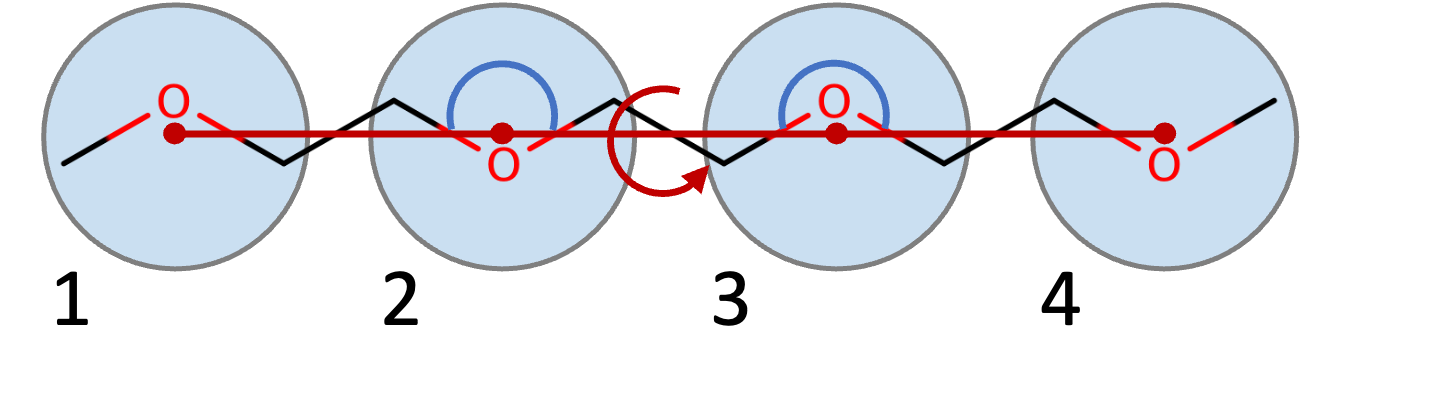
Analogously, we have 2 triplets of atoms (atoms 1-2-3 and 2-3-4 above; angles that are indicated with a blue semi-circle in the figure above). Finally, we can also add a dihedral potential between the 1-2-3-4 atoms. These potentials are analogous to the potential terms commonly used in AA force fields (OPLS, AMBER, CHARMM, etc.). However, when developing Martini coarse-grained models, the rule of thumb is “to keep things simple”: that is, do not add extra potential terms if you do not really need it.
Having decided on the bonded terms to use, they must now be defined in the itp file
under the [ bonds ], [ angles ], and [ dihedrals ].
In general, each bonded potential is defined by stating the atom number of the particles involved,
the type of potential involved, and then the parameters involved in the potential, such
as reference bond lengths/angle values or force constants. This definition is highly dependent
on the type of potentials employed and, as such, users should always reference the
GROMACS manual for specific details.
Here, we will use this example to cover the most common potentials used in defining Martini topologies.
Bonds are defined under [ bonds ] by stating the atom number of the particles involved,
the type of bond potential (in this case, type 1, a regular harmonic bond) followed by
the reference bond length and force constant.
If we use bond 1-2 as an example, your itp should look something like this:
[bonds]
; i  j  funct length    kb
  1  2   1     0.400   1000
Angles and dihedrals follow the same strategy, stating the atom number of the particles involved, the type of potential, and, in this case, the reference angle and force constant. An angle potential would look like the following:
[ angles ]
; i  j  k  funct  ref.angle force_k
  1  2  3    2      180        20
...
Fill out the other bonded terms. Let us leave the dihedral out, at least for now.
Using initial guesses for the reference bond lengths/angles and force constants you can now create a complete topology for the target molecule. These initial guesses will be improved upon in a further section by comparing the AA and CG bonded distributions and adjusting these values.
5.2) Index files and generation of target distributions
Once you have settled on the bonded terms, create an index file for the bonds with a directive [bondX] for each bond,
and which contains pairs of CG beads. For example:
[bond1]
  1  2
[bond2]
  2  3
...
and similarly for angles (with triples of CG beads) and dihedrals (with quartets). Let’s name these files
bonds.ndx, angles.ndx, and dihedrals.ndx. Write scripts that generate
distributions for all bonds, angles, and dihedrals you are interested in. For PEO4,
there are three bonds, two angles, and one dihedral, as discussed. A script is also provided, so that:
cd  PEO4-in-vacuum/5_target-distr
[create bonds.ndx, angles.ndx, and dihedrals.ndx]
bash 5_generate_target_distr.sh
will create the distributions. Inspect the folders bonds_mapped, and dihedrals_mapped for the results.
You will find each bond distributions as bonds_mapped/distr_bond_X.xvg and a summary of the mean and standard deviations
of the mapped bonds as bonds_mapped/data_bonds.txt.
For each bond, the script uses the following command (in this example, the command is applied for the first bond, whose index is 0):
echo 0 | gmx distance -f ../3_mapped/mapped.xtc -n bonds.ndx -s ../4_initial-CG/CG.tpr -oall bonds_mapped/bond_0.xvg -xvg none
gmx analyze -f bonds_mapped/bond_0.xvg -dist bonds_mapped/distr_bond_0.xvg -xvg none -bw 0.001
and similarly for the dihedral:
echo 0 | gmx angle -type dihedral -f ../3_mapped/mapped.xtc -n dihedrals.ndx -ov dihedrals_mapped/dih_0.xvg
gmx analyze -f dihedrals_mapped/dih_0.xvg -dist dihedrals_mapped/distr_dih_0.xvg -xvg none -bw 1.0
6) Create the CG simulation
We can now finalize the first take on the CG model, PEO4_take1.itp, by adding the bonded parameters discussed
at 5.1) and use the info contained in the data_bonds.txt
and data_dihedrals.txt files to come up with better guesses for the bonded parameters:
cd ../6_CG-takeCURRENT
cp ../4_initial-CG/molecule.gro      .
cp ../4_initial-CG/PEO4_initial.itp  PEO4_take1.itp
[add bonded parameters as discussed in 5.1) if not done already]
[adjust PEO4_take1.itp with input from the previous step]
bash prepare_CG_1mol_system.sh  molecule.gro  box_CG_W_eq.gro  W  1
where the command will run an energy-minimization, followed by an NPT equilibration, and by an MD run of 50 ns
(inspect the script and the various mdp files to know more) for the Martini system in water.
Once the MD is run (you will see that it is blazing fast!), you can use the index files generated for the mapped trajectory to generate the distributions of the CG trajectory:
cp ../5_target-distr/*.ndx .
bash 6_generate_CG_distr.sh
which will produce files as done by the 5_generate_target_distr.sh in the previous step but now for the CG trajectory.
7) Optimize CG bonded parameters
You can now plot the distributions against each other and compare. You can use the following scripts:
python plot_bonds_tutorial_3x1.py
The plots produced should look like the following, for bonds (AA is in blue, Martini is in red):
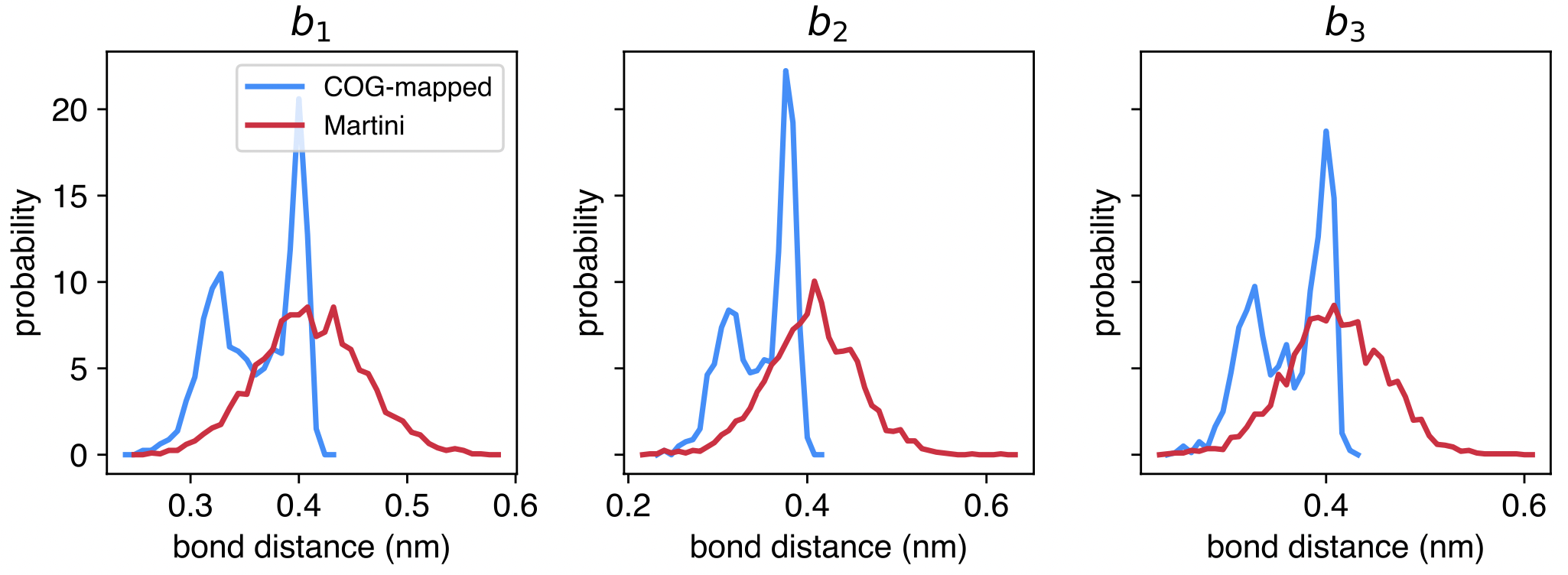
Can you plot the comparison between the angle distribution? And the dihedral?
Moreover, the agreement for the bonds is not very good in this case. Can you improve on that?
If the agreement is not satisfactory
at the first iteration - which is likely to happen - you should play with the equilibrium value and force constants in the CG itp
and iterate till satisfactory agreement is achieved.
8) Make an `.ff` file for PEO
To easily make polymers of arbitrary lengths from the parameters we just obtained,
a great option is implementing the current .itp file into an .ff file, so that we can leverage the Polyply tool [7].
The .ff file format is explained at this link.
Try to see what you should do for PEO.
Once you have a first guess, you can compare your .ff file to the one of
the PEO Martini 3 model already available in the polyply library that can be found
at this link.
References and notes
[1] P.C.T. Souza, et al., Nat. Methods 2021, 18, 382–388.
[2] R. Alessandri, et al., Adv. Theory Simul. 2022, 5, 2100391.
[3] S.J. Marrink, et al., J. Phys. Chem. B. 2007, 111, 7812-7824.
[4] W.L. Jorgensen and J. Tirado-Rives, PNAS 2005, 102, 6665; L.S. Dodda, et al., J. Phys. Chem. B, 2017, 121, 3864; L.S. Dodda, et al., Nucleic Acids Res. 2017, 45, W331.
[5] J. Barnoud, https://github.com/jbarnoud/cgbuilder.
[6] The Gromacs tool gmx traj won’t allow to choose more than one group unless one passes the flag -com. Neither -nocom or omitting the flag altogether (which should give -nocom) work.
[7] F. Grunewald, et al., Nat. Commun. 2022, 13, 68